Piecewise Developable Surface Approximation with Gauss Stylization
Project by Tobias Loch (tobias.loch@tu-berlin.de)
Input
Output
Assembling a Piecewise Developable Surface [2]
Bringing complex 3D shapes into the real world is a challenging task. While 3D printers are becoming more and more popular, they still struggle with complex shapes. To address this, we explore Piecewise Developable surfaces—locally flat surfaces, called patches, that approximate curved shapes. Those patches are easy to manufacture and assemble, due to their simple shape. An example of this can be seen on the right. Furthermore, surfaces composed of these developable pieces reduce costs and enhance quality within computer-controlled milling procedures, as demonstrated by the work of Harik et al. [5] in 2013.
In recent years there have been two approaches for approximating Piecewise Developable Surfaces. The first was introduced by Stein et al. [2] in 2018. They improved the definition of Piecewise Developability via introducing new properties of measuring developability and created an optimization technique to optimize for Piecewise Developability. In 2021 Liu and Jacobsen [1] built up on this by introducing a Stylization technique based on vertex normal preferences which they used to apply a developable style that also optimizes for the properties introduced by Stein et al.
The goal of this article is to use the optimization from Liu and Jacobsen and combine it with the face normal based Gauss Stylization from Kohlbrenner et al. [3] to create a powerful method for accurate and visually captivating surface approximation. We detail the technique, algorithms, and results, showcasing how the approach bridges the gap between practical efficiency and complex shape representation.
Developability
Piecewise Developability refers to a geometric modeling approach where a complex surface is approximated using a collection of smaller developable patches. Developable patches are surfaces that can be flattened onto a plane without stretching or tearing, like rolling out a piece of paper. In the discrete context we can define flattenability as follows:
A triangulated surface is flattenable if the angle sum equals \(2\pi\) at every vertex.
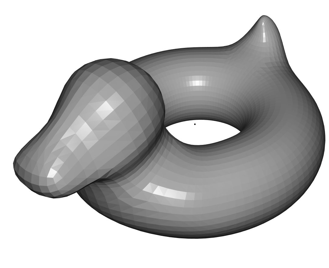
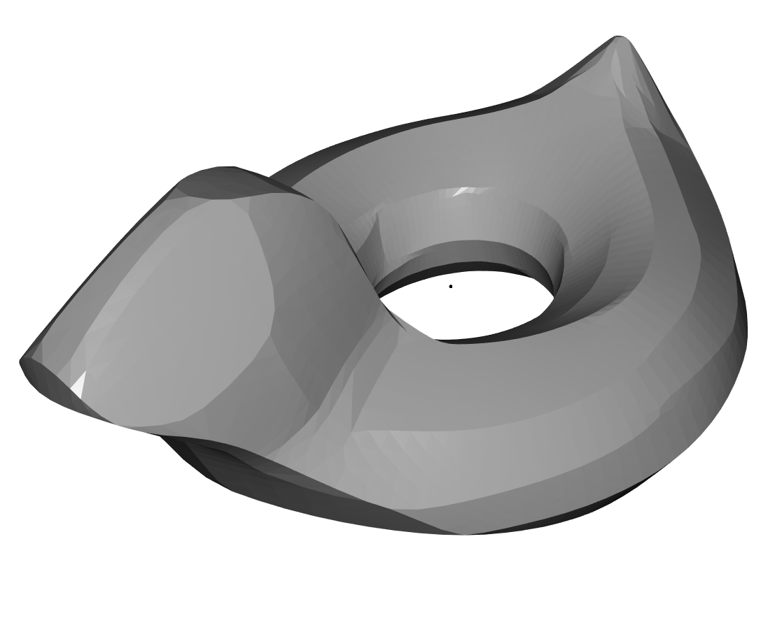
Due to the flattenability inherent in the patches of a Piecewise Developable surface, the curvature focuses primarily on the transitions between patches, while the patches themselves are low curved. This is illustrated in the images below.
Original
Piecewise Developable
A discrete ruling line is a line that connects two vertices of the mesh and is straight on the surface. A surface is discretely ruled if every vertex is contained in a discrete ruling line such that all that ruling lines are parallel.
Comparing different flattenable surfaces [2]
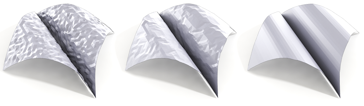
Flattening out a Hinge
A Vertex is a hinge if the normals of its incident triangles are contained in a common plane and does not self intersect.
By optimizing for hinges, surfaces can be both discretely ruled and flattenable, which balances between these two important characteristics.
Stein et al. demonstrated that hinges consistently lead to vertices with incident triangles partitioned into exactly two edge-connected regions, each characterized by constant normals. This attribute ensures easy flattening, as the normals are already in a common plane. Moreover, hinges imply a distinct ruling line, for the three vertices adjacent to both regions. Furthermore, the results from Stein et al. show that optimizing for such leads to clearly ruled surfaces.
In summary, if all vertices of a mesh are hinges, then the surface is Piecewise Developable.
Next we will introduce the algorithm that we use to optimize for hinges.
Gauss Stylization
Gauss Stylization [3] is a tequnique that changes the shape of a triangle surface mesh while keeping its overall appearance similar. In short, it maximises for given face normal directions, while penalising non-rigid transformations.
To achieve this the following energy is minimized: $$ E_G^*(V,R,n^*,e^*) = E_{ARAP}(V,\{R_i\}) - \mu \sum_{f\in F} g(n^*_f) +\lambda \sum_{(i,j)\in E} \frac{w_{ij}}{2} \|e_{ij} - e^*_{ij}\|^2, \\\textrm{s.t. } {n^*_f}^T e^*_{ij} = 0 \textrm{ with } (i,j) \in f $$
| \(E_{ARAP}(V,\{R_i\})\) | This is the As-Rigid-As-Possible (ARAP) energy term which penalises non-rigid transformations, that shear or stretch the mesh. \(V\) are the vertex positions and \(R\) are the local rotations. |
| \(\mu\sum_{f\in \mathcal{F}} g(n^*_f)\) | This term enforces the face normals \(n^*_f\) to be aligned with the given normal preferences, which are defined by \(g\). Increasing the parameter \(\mu\) leads to faster convergence of the algorithm, but can also result in more deformations, due to the fact that it decreases the influence of the \(E_{ARAP}\) energy. \(\mathcal{F}\) is the set of faces. |
| \(\lambda\sum_{(i,j)\in \mathcal{E}} \frac{w_{ij}}{2} \|e_{ij} - e^*_{ij}\|^2\) | This regularization term ensures that normals of neighboring faces are not optimized independently. Increasing the parameter \(\lambda\) results in stronger stylization. \(e^*_{ij}\) are the desired edge vectors, \(e_{ij}\) the original ones, \(w_{ij}\) are edge weights and \(\mathcal{E}\) is the set of edges. |
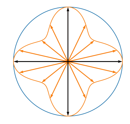
Example preference function [3]
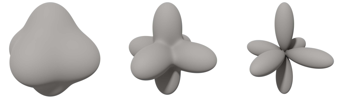
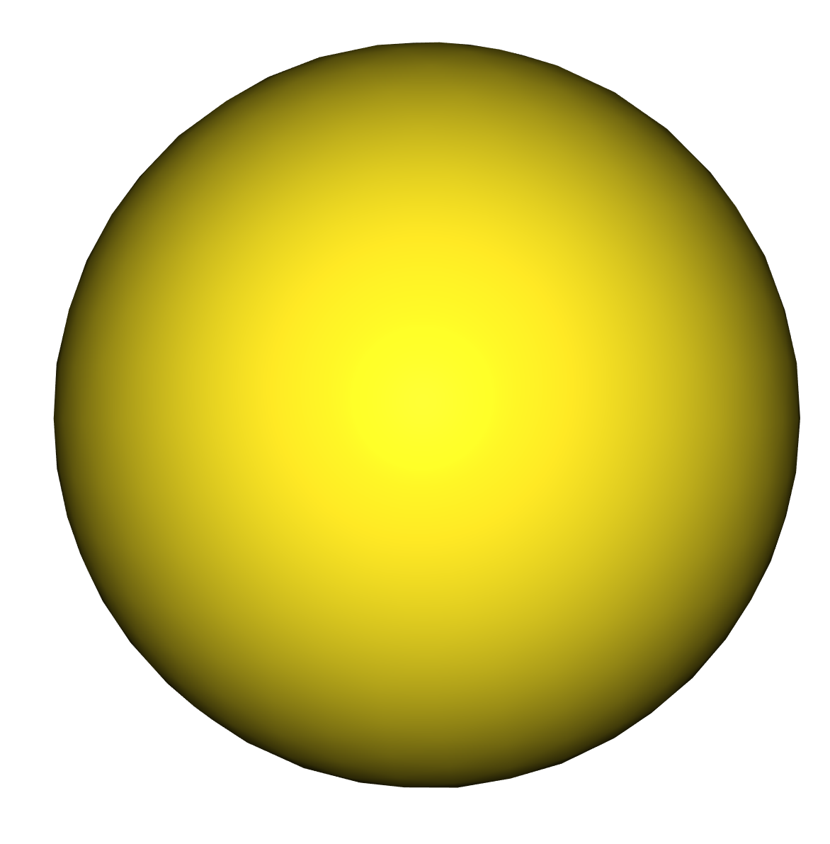
\(g\) is the preference function. It is modeled as a mixture of Gaussians. The preferences can be also defined face wise, which we will use later. \(g\) is defined as follows: $$ g(x) = \sum_k w_k \exp(\sigma x^T n_k) $$ \(n_k\) are the normal preferences and \(w_k\) are their weights. We always set the weights to 1, because we only have one preference per face. Therefore, they can be ignored. \(\sigma\) is a parameter that controls the width of the Gaussians. A high \(\sigma\) allows more deviation from the normal preferences. An example is shown on the right.
The minimization of the energy function is done via combining the ARAP energy minimization [6] with an Alternating Direction Method of Multipliers (ADMM) [7]. \(R\) and \(V\) are optimized according to the ARAP approach while \(e^*\) and \(n^*\) are optimized via ADMM. The number \(N\) of ADMM iterations has to be set initially. Kohlbrenner et al. pointed out that one iteration is in most cases enough. Therefore, we set \(N=1\) by default. For more details on Gauss Stylization view [3] and [6]
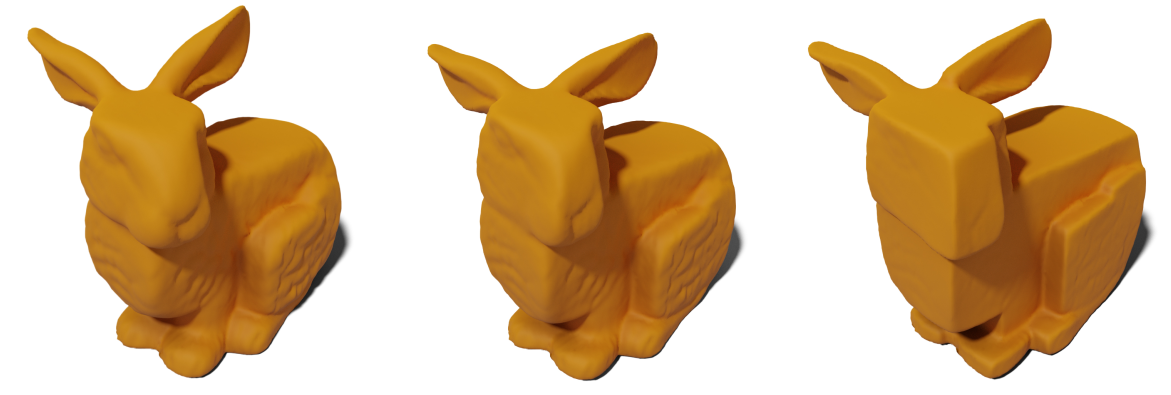
Some results from this algorithm applied on the Stanford Bunny can be seen below.
An Example of Gauss Stylization [3]
We now want to use this algorithm to apply a style that makes a given mesh Piecewise Developable. Therefore we need to find normal preferences that optimize for hinges.
Finding Normal Preferences
The following algorithm is based on the paper from Liu and Jacobsen [1]. Their approach stylizes triangle meshes via vertex normal preferences and based on this they developed a technique to make meshes piecewise developable. We want to combine their technique with the face normal based Gauss Stylization algorithm. Due to the fact, that the algorithm applies the style iteratively, the normal preferences are generated before each iteration. We calculate a single normal preference for each face individually. The algorithm looks as follows:
| \(V\) | Vertices of the triangle mesh |
| \(F\) | Faces of the triangle mesh |
| \(N\) | Matrix containing normals for each face \(f\in F\) |
| \(\text{adj}(v)\) | Faces around a vertex \(v\in V\) |
| \(N_{\text{adj}(v)}\) | Matrix containing the face normals around a vertex \(v \in V\) |
| \(\theta \in \mathbb{Q}\) | Threshold to control the number of collapses |
| \(P_f\) | Face normal preferences for each face \(f \in F\) |
For each \(v\in V\) // Calculate the normal preference for a single Vertex \(v\)
Calculate the Eigenvalues \(\lambda_1\), \(\lambda_2\) and \(\lambda_3\) with \(\lambda_1 < \lambda_2 < \lambda_3\) and \(w_i\) its corresponding eigenvectors of \(C\)
// first principle component = eigenvector with largest eigenvalue
If \(\lambda_2 < \theta\) then
// Project the face normals onto the first or the first two principle components
For each \(f\in\) \(\text{adj}(v)\)
For each \(f\in F\) // Average the generated Preferences
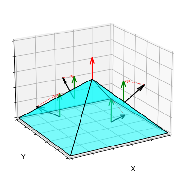
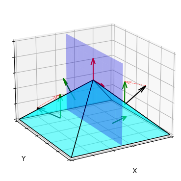
In the first part of the algorithm, we calculate normal preferences for each vertex \(v\), that are in a common plane (hinge). To do so it performs a Principle Component Analysis on the face normals around \(v\). It then projects these face normals either onto the first or first two principle components dependent on a threshold \(\theta\). If the second eigenvalue is smaller than \(\theta\), then the face normals are projected onto the first principle component. Otherwise they are projected onto the first two principle components. This value should control the number of crashes the approximation has.
In the second part of the algorithm, we average the generated normal preferences facewise. Due to the fact that each face has at most three adjacent vertices, we get at most three preferences per face from the step before. We did this by simply adding up the vectors and then normalizing them in the end.
Example of a single iteration of the algorithm
Implementation
We forked the implementation provided by Kohlbrenner et al. [3] for Gauss Stylization which provided a modeling interface using the igl library. We changed the implementation such that only the relevant parts remained and implemented the algorithm from the last section. The code is in C++ and provided at https://gitlab.cg.tu-berlin.de/sempro/cgp-ss23-gauss-stylization-developable.
Here is a short summary of the parameters that have to be set for modeling:
| \(N\) | The number of ADMM iteration steps. Most of the time a value of \(1\) is enough, but for faster convergence this can be increased. |
| \(\lambda\) | The weight of the regularization term of the Gauss Stylization Energy. This parameter controls how strong the stylization is after convergence. By default we set it to \(3000\). |
| \(\mu\) | The weight of the preference function term of the Gauss Stylization Energy. Increasing this value accelerates the convergence, but can lead to deformations due to decreasing the influence of the ARAP energy in each iteration. We used most of the time a value of \(1\). |
| \(\sigma\) | The width of the Gaussians used for the preference function. Higher values of \(\sigma\) allows more deviation from the normal preferences. This can sometimes result in clearer patches. By default we set this value to \(10\). For meshes with less faces we recommend decreasing this, to have less deformations. |
| \(\theta\) | The threshold for the PCA. This value controls how many crashes the algorithm has. Lower values lead to more patches. A good value is around \(0.005\) to \(0.001\). A value greater than \(1\) leads to no patches at all, because all faces are projected onto the first principle component. |
Results
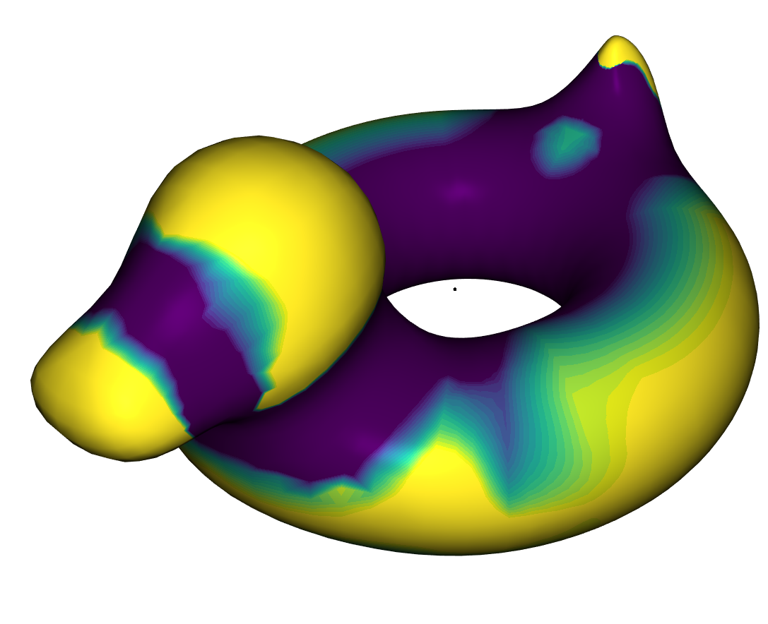
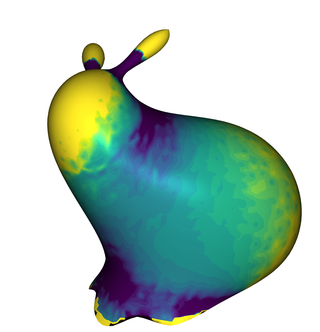
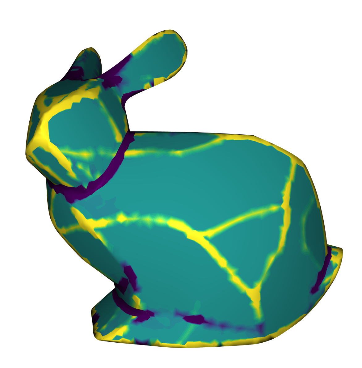
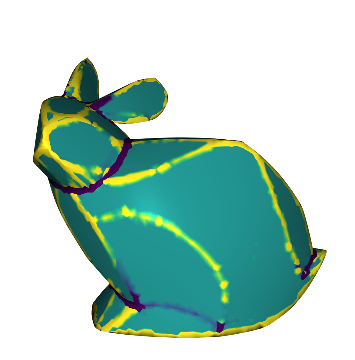
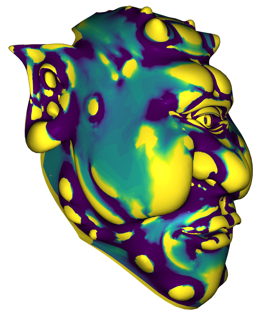
We use the Gaussian Curvature to measure the performance of the algorithm. The Gaussian Curvature is defined on a continous surface as the product of the two principle curvatures. On discrete surfaces it can be defined via the angle deficit and is then calculated as follows: $$k(v_i) = 2 \pi - \sum_{j \in N(i)} \theta_{ij}$$ Here \(N(i)\) are the adjacent triangles of the vertex \(v_i\) and \(\theta_{ij}\) is the angle at vertex \(i\) and triangle \(j\). In our implementation it is calculated according to the igl library which also normalised it over the area. For more details view [4].
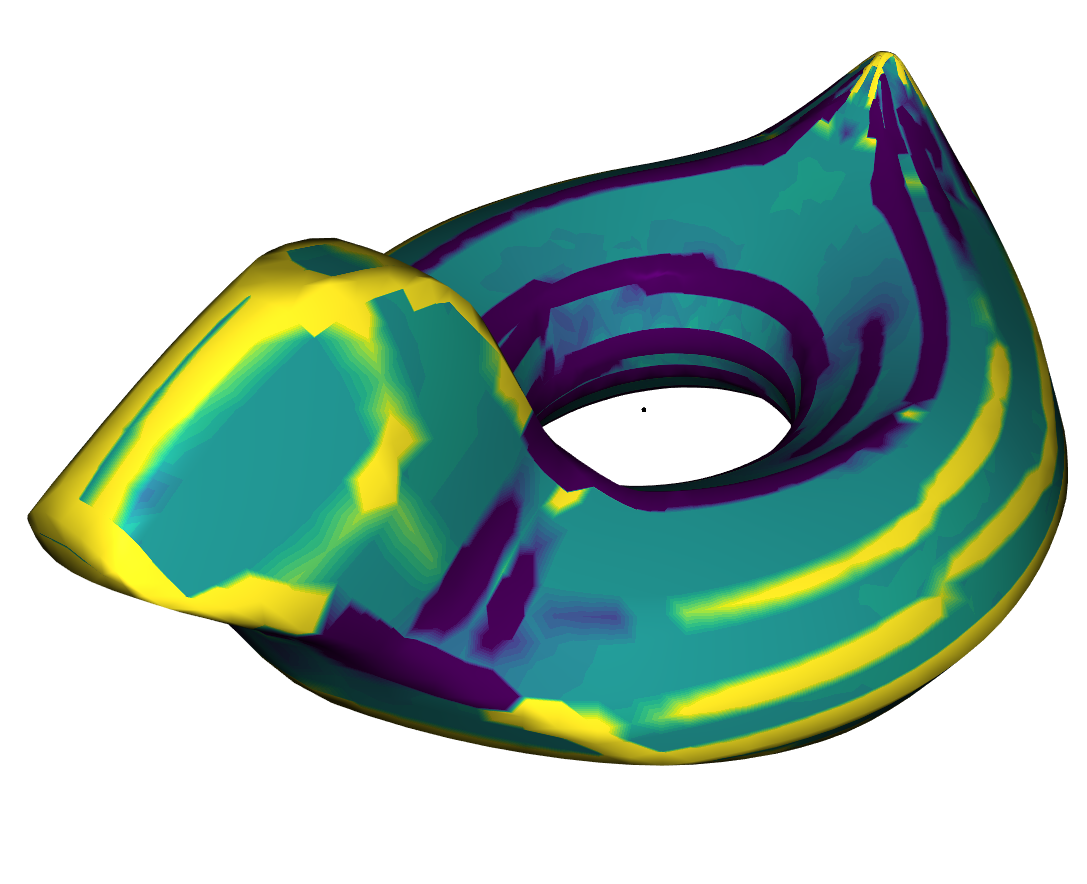
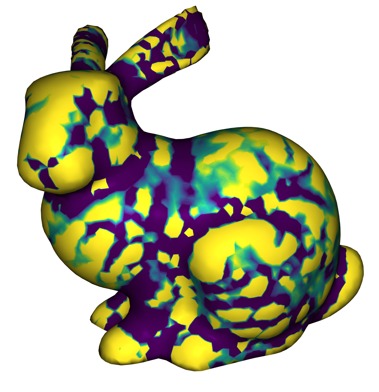
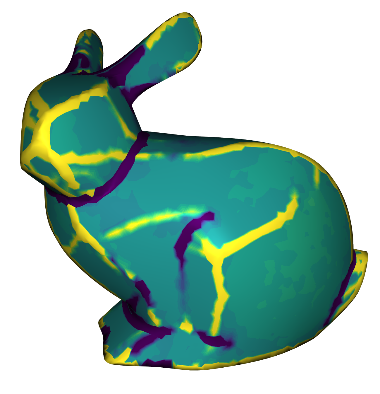
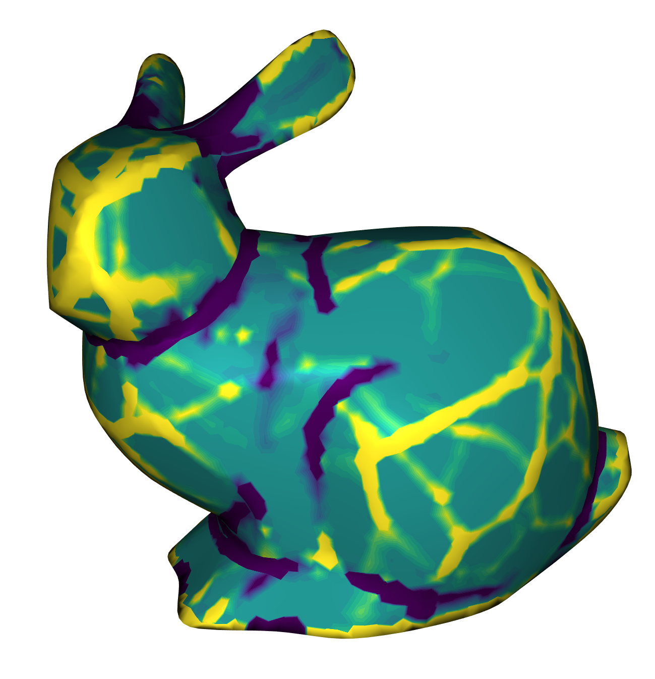
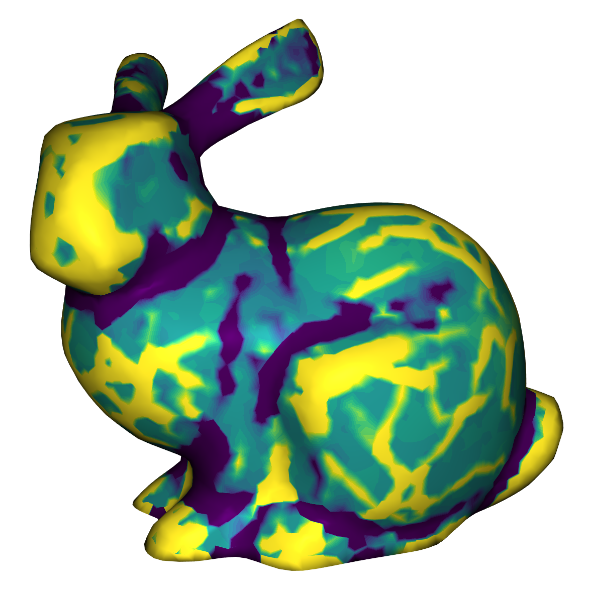
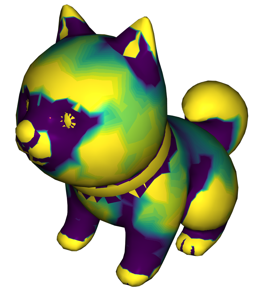
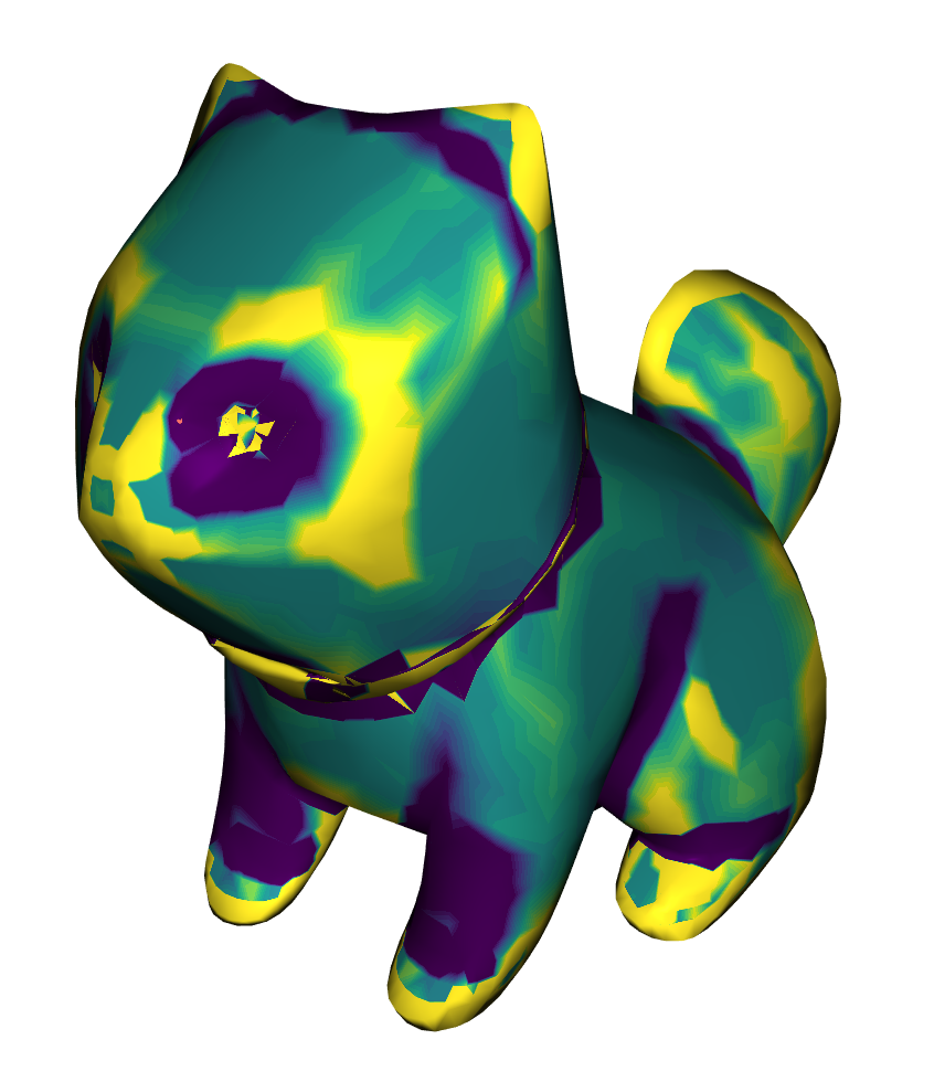
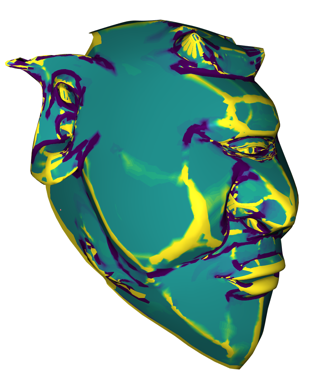
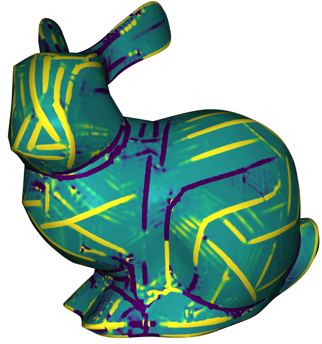
We used the Viridis color map to visualize the Gaussian Curvature on a surface. Blue means bent inward, turquoise means flat and yellow means bent outward. When the absolute of the curvature is higher than a given maximum \(\omega\), then we capped it at that value. This was useful to see more details. On all tests we applied \(1000\) iterations of the algorithm. The following images show the Gaussian Curvature of the original Stanford Bunny and the Gaussian Curvature of the approximated Stanford Bunny with \(\theta = 0.0025, \lambda=10^3, \sigma=10\) and \( \mu=1\). In the visualisation we set \(\omega=2^4\). Clicking on the images disables the curvature color map.
Input
Output
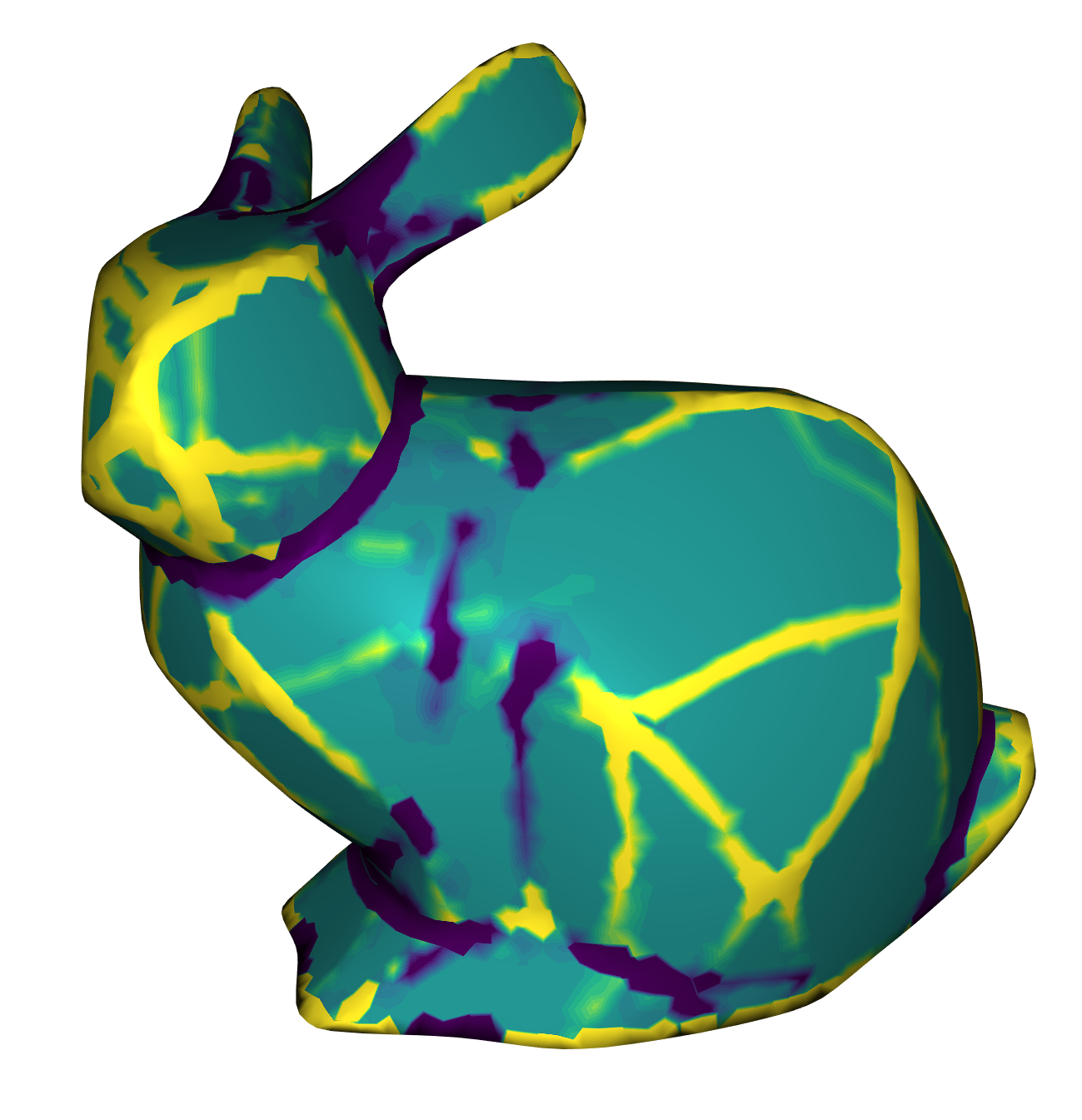
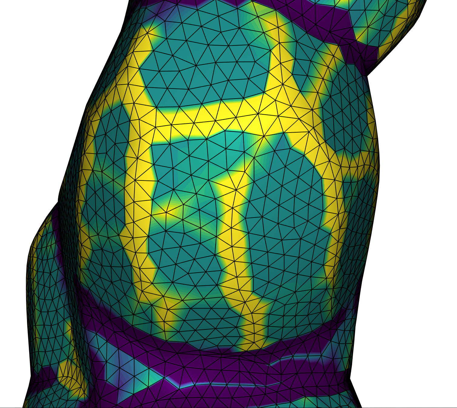
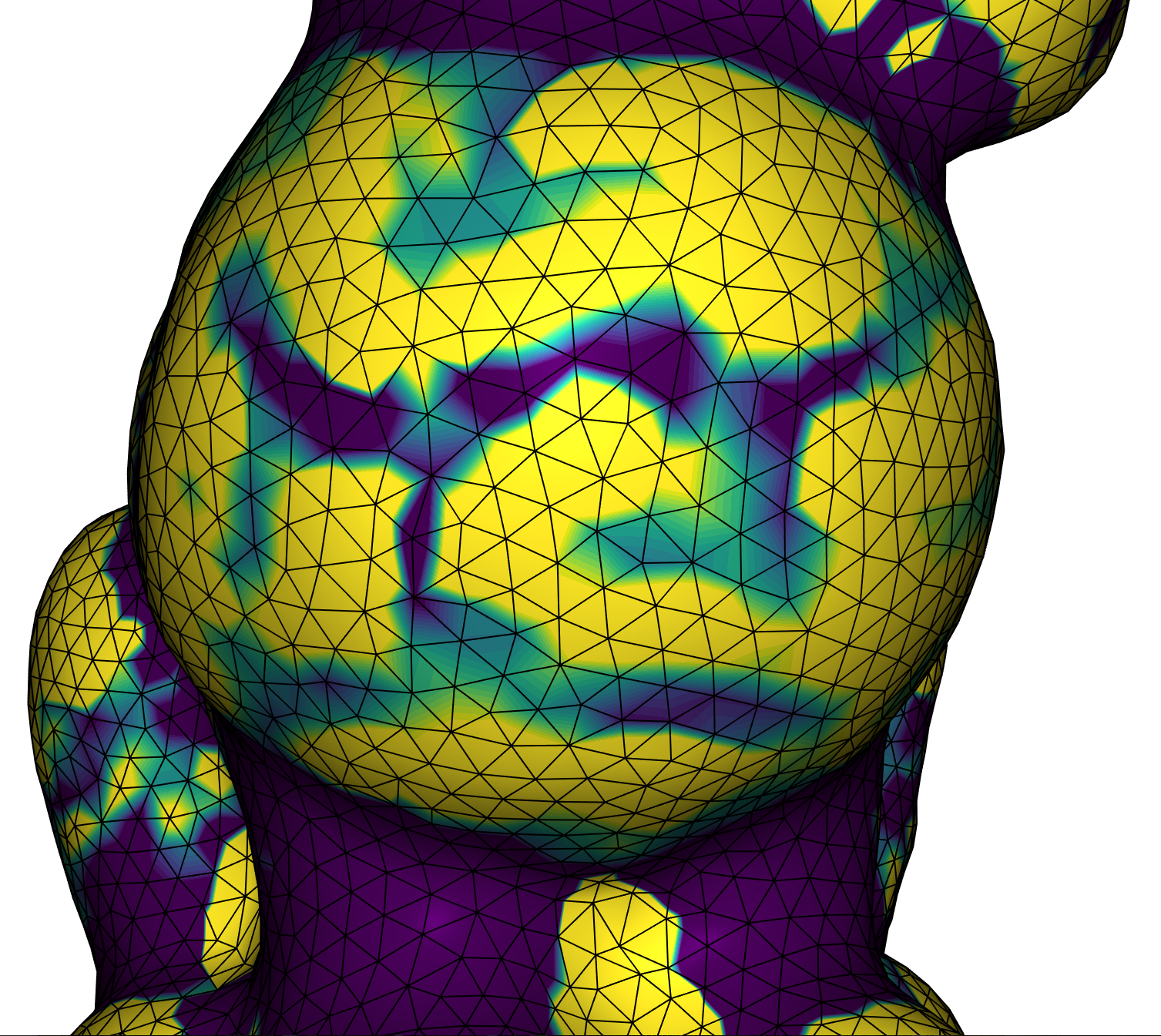
The Curvature concentrates onto some edges on the output mesh. Those are the transitions of the patches. On the patches the curvature is mostly turquoise which means that it is low curved there. While the patches remain flat the algorithm does not guarantee them to be discretely ruled. This can be seen on the closeup image where the edge lines are painted black. This is probably due to the fact that the ARAP optimization penalises changing the topology of the mesh.
Next we compared the influence of \(\theta\) onto the algorithm. Below are some images which show the results for different values of \(\theta\).
\(\theta = 1\)
\(\theta = 0.005\)
\(\theta = 0.001\)
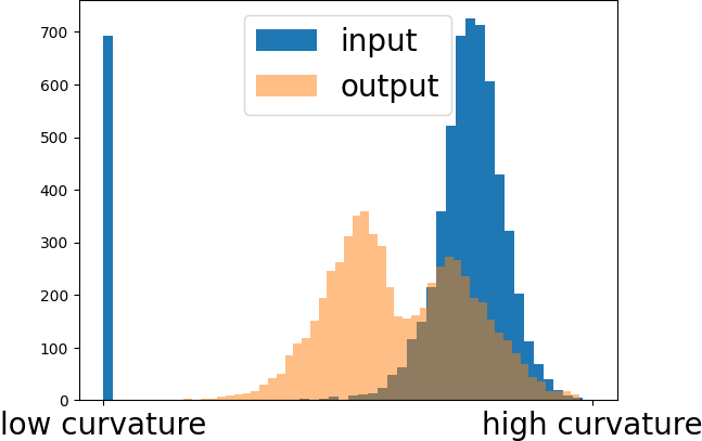
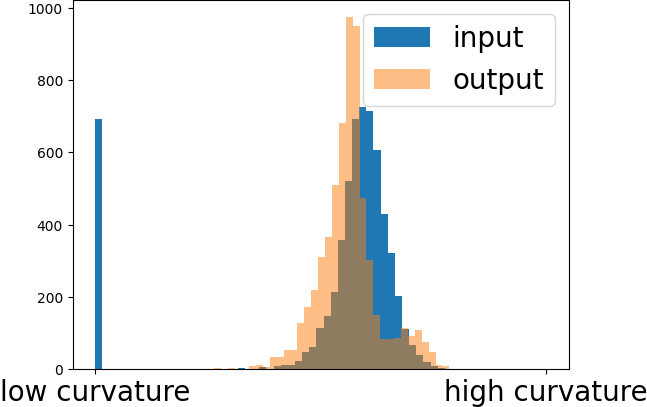
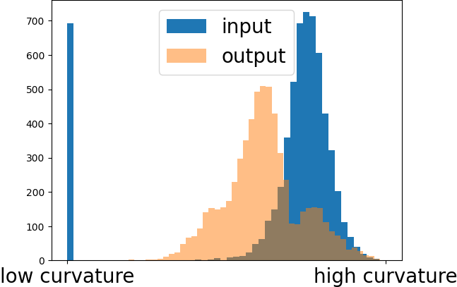
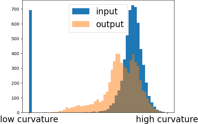
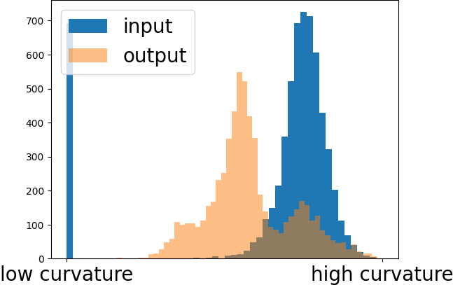
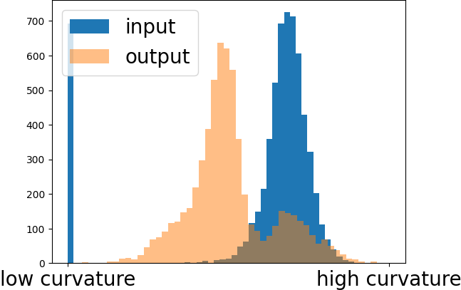
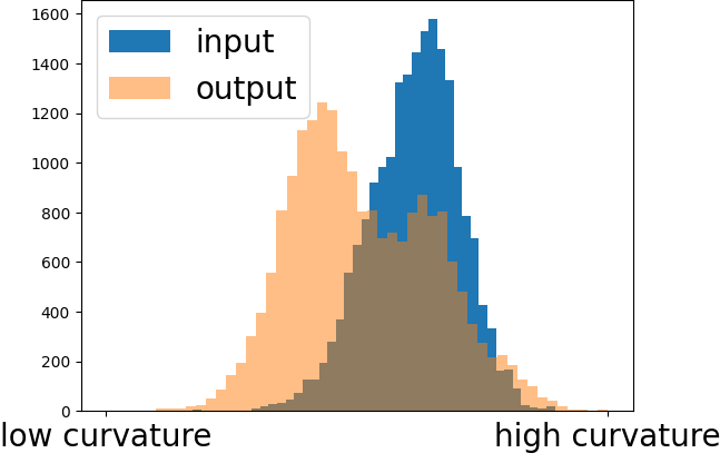
It is clear to see how \(\theta\) influences the generation of patches. When it decreases more crashes happen and therefore more and smaller patches are generated. On the left we never project the face normals onto the first two principle components and therefore we have only one preference normal around each vertex. This results in smoothing the mesh. Below the images we plotted a histogram with logarithmic scale of the Gaussian Curvature magnitude. It is clear to see that the curvature of most vertices decreases. This is due to the fact that it is more concentrated on the transition of the patches, while the patches itself are mainly flat. The spike blue on the left of the histograms is the curvature of the ground plane of the bunny, which is slightly changed during the optimization.
Next we compared the influence of changing sigma. Below are some images which show the results for different values of sigma with \(\theta=0.0025\). The other parameters are unchanged.
\(\sigma = 1\)
\(\sigma = 20\)
\(\sigma = 40\)
Increasing \(\sigma\) leads to clearer patches. If it is high, then the mesh deforms, which is visible on the right image. This is due to the fact that the width of the Gaussians is too large and therefore tolerates large deviations from the face normal preferences. While we double \(\sigma\) between the middle and the right image, the curvature in the histogram only changes slightly. Therefore, a value up to 20 leads to good results in this situation. From our experience we recommend setting \(\sigma\) to 4 or 10.
Below you can see more results of the algorithm on different meshes.
Input
Output
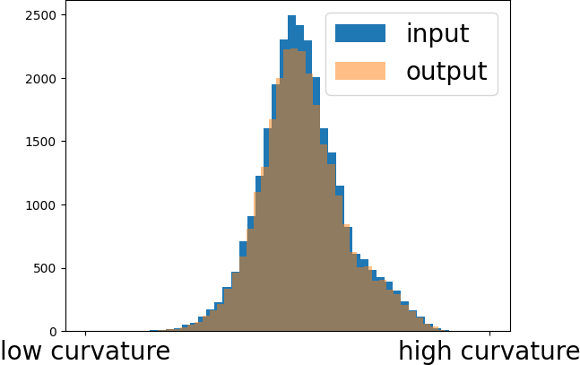
Gauss Curvature Histogram
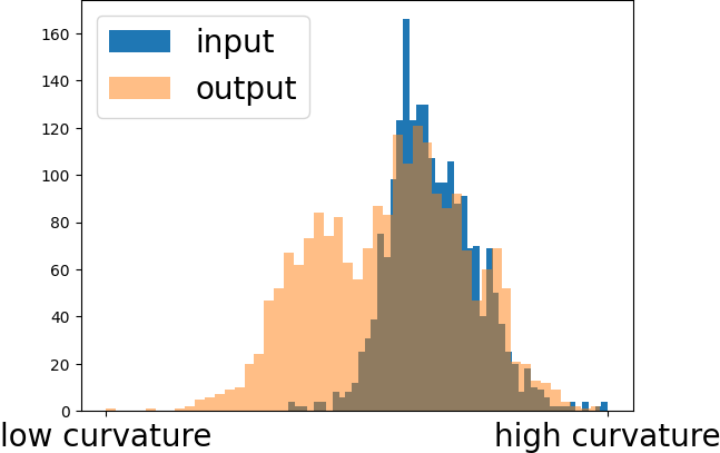
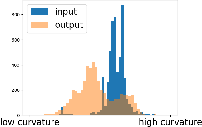
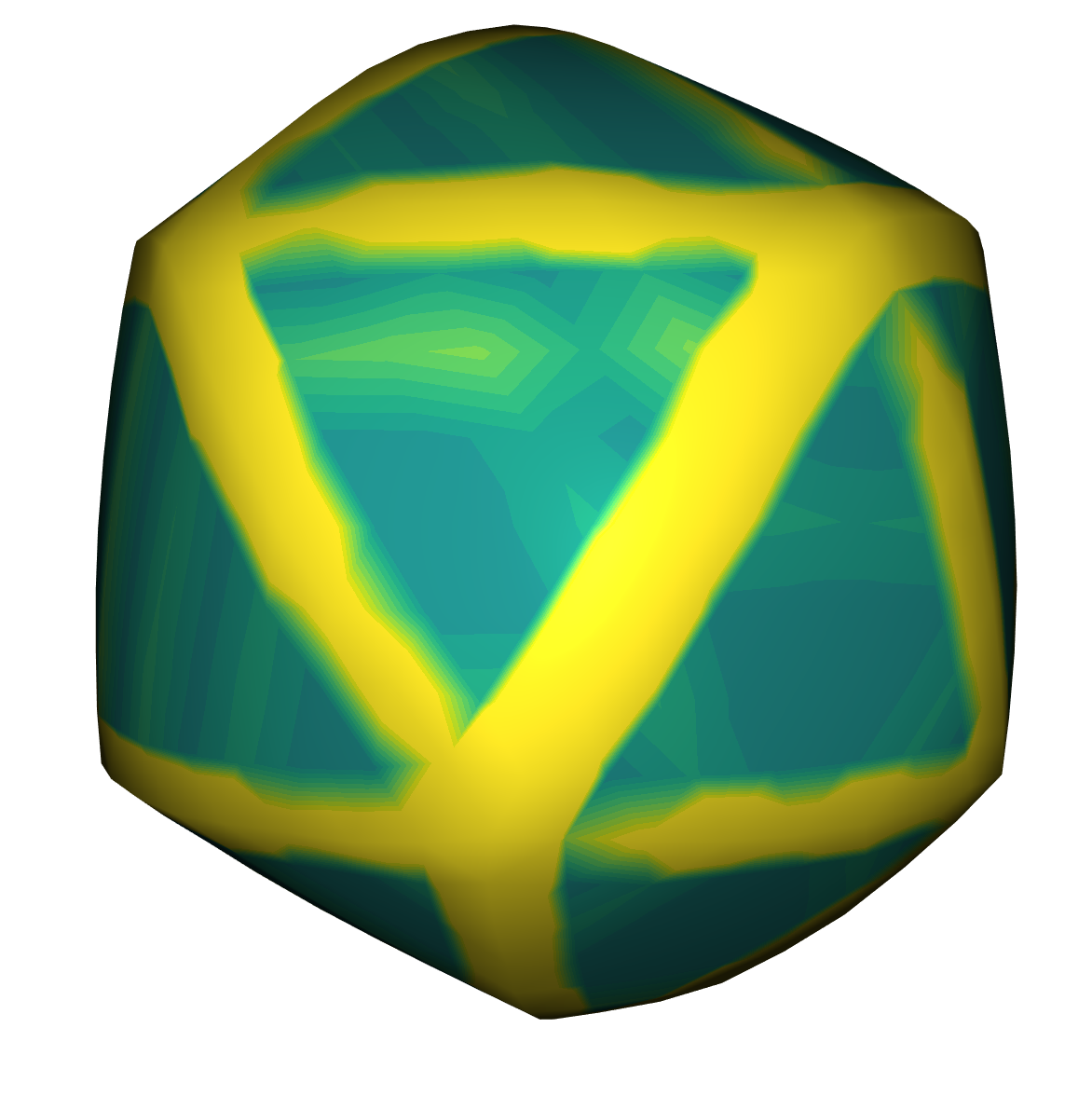
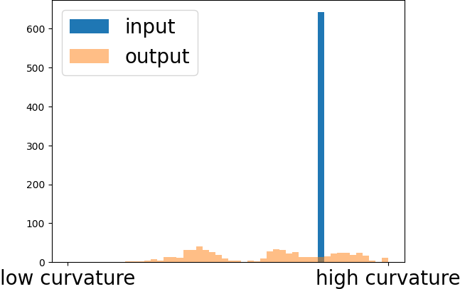
The curvature decreased on all meshes above. Also, the generation of patches can be seen. Next we applied the algorithm on a mesh generated by Stein et al. which is already Piecewise Developable.

There is only a slight change visible. This shows that the algorithm is able to preserve the developability of a mesh. In comparision to the bunny we generated from the beginning of the section it is notable that the bunny from Stein et al. has less complex transitions between the patches.
Conclusion
In summary, the presented implementation offers a straightforward tool of reducing mesh curvature and approximating Piecewise Developable surfaces. However, it's important to acknowledge certain drawbacks. Notably, the patches are not guaranteed to be discretely ruled. Also, the transitions between patches are complex. This can pose challenges in the manufacturing phase. Approximating the patches with discretely ruled surfaces could be a future research direction.
It would be interesting to see how easy the mesh can be printed out and assembled together. The implementation could be improved by implementing algorithms for identifying the patches and printing them out. The patches for example could be identified via a clustering algorithm that puts two neighboring vertices into the same cluster if they have a similar normal depending on a threshold. The set of patches then have to be flattened out for printing which can be done for example using the Gauss Stylization approach.
Furthermore comparing the running time between the three different approaches would be interesting. Also some more experiments could be done to see how the different parameters influence the results.
In conclusion, our study demonstrates the potential of the Gauss Stylization method for developable surface approximation. While challenges exist, advancements in patch identification, patch approximation, printing feasibility and parameter variation stand as promising directions for future research in this domain.
References
- [1] Hsueh-Ti Derek Liu and Alec Jacobson. "Normal-Driven Spherical Shape Analogies". In: CoRR abs/2104.11993 (2021). arXiv: 2104.11993. url: https://arxiv.org/abs/2104.11993.
- [2] Oded Stein, Eitan Grinspun, and Keenan Crane. "Developability of Triangle Meshes". In: ACM Trans. Graph. 37.4 (2018).
- [3] Maximilian Kohlbrenner, Ugo Finnendahl, Tobias Djuren and Marc Alexa "Gauss Stylization: Interactive Artistic Mesh Modeling based on Preferred Surface Normals". In: Computer Graphics Forum (2021). issn: 1467-8659. doi: 10.1111/cgf.14355.
- [4] https://libigl.github.io/tutorial/#gaussian-curvature
- [5] Harik, Ramy F., Hu Gong, and Alain Bernard "5-Axis Flank Milling: A State-of-the-Art Review." In: Computer-Aided Design (2013). url: https://doi.org/10.1016/j.cad.2012.08.004.
- [6] Olga Sorkine and Marc Alexa. “As-Rigid-As-Possible Surface Modeling”. In: Proceedings of EUROGRAPHICS/ACM SIGGRAPH Symposium on Geometry Processing (2007). pp. 109–116
- [7] Boyd, Stephen & Parikh, Neal & Chu, Eric & Peleato, Borja & Eckstein, Jonathan. Distributed Optimization and Statistical Learning via the Alternating Direction Method of Multipliers. In: Foundations and Trends in Machine Learning (2011). 3. 1-122. doi: 10.1561/2200000016.